The Cox Proportional Hazards Model and Its Characteristics

---

The Formula for the Cox PH Model

The Cox PH model is usually written in terms of the hazard model formula shown here below. This model gives an expression for the hazard at time $t$ for an individual with a given specification of a set of explanatory variables denoted by the bold X. That is, the bold X represents a collection (sometimes called a "vector") of predictor variables that is being modeled to predict an individual's hazard.

$$h(t, \mathbf{X}) = h_o(t)e^{\sum_{i=1}^{p}\beta_iX_i}$$

$$\mathbf{X}=(X_1,X_2,...,X_p)$$

where $X_1$ through $X_p$ are explanatory/predictor variables

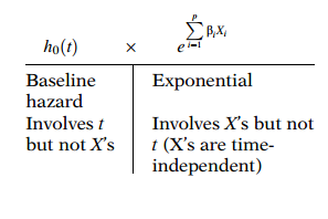
The Cox model formula says that the hazard at time $t$ is the product of two quantities. The first of these, $h_0(t)$, is called the baseline hazard function. The second quantity is the exponential expression $e$ to the linear sum of $\beta_iX_i$, where the sum is over the p explanatory $X$ variables.

An important feature of this formula, which concerns the proportional hazards (PH) assumption, is that the baseline hazard is a function of $t$, but does not involve the $X$'s. In contrast, the exponential expression shown here, involves the $X$'s, but does not involve t. The $X$'s here are called time-independent $X$'s.

$X$'s involving $t$: time-dependent

Requires extended Cox model (no PH)

It is possible, nevertheless, to consider $X$'s which do involve $t$. Such $X$'s are called time-dependent variables. If time-dependent variables are considered, the Cox model form may still be used, but such a model no longer satisfies the PH assumption, and is called the extended Cox model.

A time-independent variable is defined to be any variable whose value for a given individual does not change over time. Examples are SEX and smoking status (SMK). Note, however, that a person's smoking status may actually change over time, but for purposes of the analysis, the SMK variable is assumed not to change once it is measured, so that only one value per individual is used.

Definition

Time-independent variable: Values for a given individual do not change over time; e.g., SEX and SMK

Also note that although variables like AGE and weight (WGT) change over time, it may be appropriate to treat such variables as time-independent in the analysis if their values do not change much over time or if the effect of such variables on survival risk depends essentially on the value at only one measurement.

The Cox model formula has the property that if all the $X$'s are equal to zero, the formula reduces to the baseline hazard function. That is, the exponential part of the formula becomes $e$ to the zero, which is 1. This property of the Cox model is the reason why $h_0(t)$ is called the baseline function.

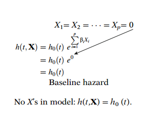
Or, from a slightly different perspective, the Cox model reduces to the baseline hazard when no $X$'s are in the model. Thus, $h_0(t)$ may be considered as a starting or "baseline" version of the hazard function, prior to considering any of the $X$'s.

Another important property of the Cox model is that the baseline hazard, $h_0(t)$, is an unspecified function. It is this property that makes the Cox model a semiparametric model.

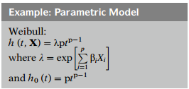
In contrast, a parametric model is one whose functional form is completely specified, except for the values of the unknown parameters. For example, the Weibull hazard model is a parametric model and has the form shown here, where the unknown parameters are $\lambda$, $p$, and the $\beta_i$'s. Note that for the Weibull model, $h_0(t)$ is given by $\lambda pt^{p-1}$

---

ML Estimation of the Cox PH Model

We now describe how estimates are obtained for the parameters of the Cox model. The parameters are the $\beta$'s in the general Cox model formula shown here. The corresponding estimates of these parameters are called maximum likelihood (ML) estimates and are denoted as $\hat{\beta}_i$.

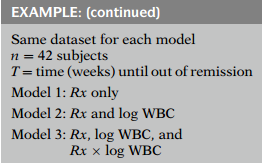
As an example of ML estimates, we consider once again the computer output for one of the models (model 2) fitted previously from remission data on 42 leukemia patients. The Cox model for this example involves two parameters, one being the coefficient of the treatment variable (denoted here as $Rx$) and the other being the coefficient of the $log \mathrm{WBC}$ variable. The expression for this model is shown at the left, which contains the estimated coefficients $1.294$ for $Rx$ and $1.604$ for log white blood cell count.

As with logistic regression,the ML estimates of the Cox model parameters are derived by maximizing a likelihood function, usually denoted as $L$. The likelihood function is a mathematical expression which describes the joint probability of obtaining the data actually observed on the subjects in the study as a function of the unknown parameters (the $\beta$'s) in the model being considered. $L$ is sometimes written notationally as $L(\beta)$ where $\beta$ denotes the collection of unknown parameters.

The expression for the likelihood is developed at the end of the chapter. However, we give a brief overview below.

The formula for the Cox model likelihood function is actually called a "partial" likelihood function rather than a (complete) likelihood function. The term "partial" likelihood is used because the likelihood formula considers probabilities only for those subjects who fail, and does not explicitly consider probabilities for those subjects who are censored. Thus the likelihood for the Cox model does not consider probabilities for all subjects, and so it is called a "partial" likelihood.

---

Computing the Hazard Ratio

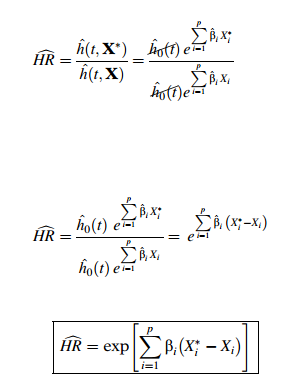
In general, a hazard ratio (HR) is defined as the hazard for one individual divided by the hazard for a different individual. The two individuals being compared can be distinguished by their values for the set of predictors, that is, the X's. We can write the hazard ratio as the estimate of $h(t,\mathbf{X}^*)$ divided by the estimate of $h(t,\mathbf{X})$, where $\mathbf{X}^*$ denotes the set of predictors for one individual, and $\mathbf{X}$ denotes the set of predictors for the other individual.

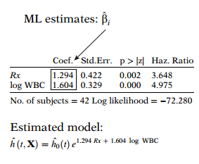
Note that, as with an odds ratio, it is easier to interpret an HR that exceeds the null value of 1 than an HR that is less than 1. Thus, the $X$'s are typically coded so that group with the larger hazard corresponds to $\mathbf{X}^*$, and the group with the smaller hazard corresponds to $\mathbf{X}$. As an example, for the remission data described previously, the placebo group is coded as $X^*_1=1$, and the treatment group is coded as $X_1=0$.

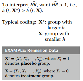
We now obtain an expression for the HR formula in terms of the regression coefficients by substituting the Coxmodel formula into the numerator and denominator of the hazard ratio expression. This substitution is shown here. Notice that the only difference in the numerator and denominator are the $X^*$'s versus the $X$'s. Notice also that the baseline hazards will cancel out.

Example1

Suppose, for example, there is only one $X$ variable of interest, $X_1$, which denotes (0,1) exposure status, so that $p = 1$. Then, the hazard ratio comparing exposed to unexposed persons is obtained by letting $X_1^* = 1$ and $X_1 = 0$ in the hazard ratio formula. The estimated hazard ratio then becomes $e$ to the quantity $\beta_1$ "hat" times 1 minus 0, which simplifies to $e$ to the $\beta_1$ "hat."

Recall the remission data printout for Model 1, which contains only the $Rx$ variable, again shown here. Then the estimated hazard ratio is obtained by exponentiating the coefficient 1.509, which gives the value 4.523 shown in the HR column of the output.

Example2

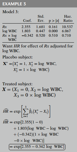
We now give a second example which illustrates how to compute a hazard ratio when the model does contain product terms. We consider the printout for Model 3 of the remission data shown here.

To obtain the hazard ratio for the effect of $R x$ adjusted for $\log$ WBC using Model 3, we consider $\mathbf{X}^*$ and $\mathbf{X}$ vectors which have three components, one for each variable in the model. The $\mathbf{X}^*$ vector, which denotes a placebo subject, has components $X_1^*=1, X_2^*=\log$ WBC and $1 \times \log$ WBC. The $\mathbf{X}$ vector, which denotes a treated subject, has components $X_1=0, X_2=$ $\log$ WBC and $X_3=0 \times \log$ WBC. Note again that, as with the previous example, the value for log WBC is treated as fixed, though unspecified. Using the general formula for the hazard ratio, we must now compute the exponential of the sum of three quantities, corresponding to the three variables in the model. Substituting the values from the printout and the values of the vectors $\mathbf{X}^*$ and $\mathbf{X}$ into this formula, we obtain the exponential expression shown here. Using algebra, this expression simplifies to the exponential of 2.355 minus 0.342 times log WBC.